Covariance convergence given new data points.
The problem
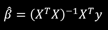
I recently read a paper on distributed multivariate linear regression. This paper essentially deals with the problem of when to update the global multivariate linear regression model in a distributed system, when the observations available to the system arrive in different computer nodes, at different times and, usually, at different rates. In the monolithic, single node case, the problem has of course been solved in closed form, since for dependent variables y and design matrix X with examples in rows, the parameter vector β can be found as per:
This is a good paper, and anybody with an interest in distributed systems and / or linear algebra should probably read it. One of the interesting things (for me) was the authors' explanation that, as more data arrives at the distributed nodes, a certain constraint on the spectral norm of a matrix product that contains information about a node's data becomes harder to satisfy. It was not clear to me why this was the case and, in the process of convincing myself, I discovered something that is probably obvious to everybody else in the world, yet I still opted to make a blog post about it, because why the hell not.
When designing any data sensor, it is reasonable to assume that the incoming multivariate data tuples will all have a non-trivial covariance. For example, in the case of two-dimensional data, it is reasonable to assume that all the incoming data points will not all lie on a straight line (which denotes full inter-dimensional correlation in the two-dimensional case). In fact, it is reasonable to assume that as more data tuples arrive, the covariance of the entire data tends to increase. We will examine this assumption again in this text, and we will see that it does not always hold water.
This hypothesized increase in the data's covariance can be mathematically captured by the spectral (or "operator") norm of the data's covariance matrix. For symmetric matrices, such as the covariance matrix, the spectral norm is equal to the largest absolute eigenvalue of the matrix. If a matrix is viewed as a linear operator in multi-dimensional cartesian space, its largest absolute eigenvalue tells us how much the matrix can "stretch" a vector in the space. So it gives us an essence of how "big" the matrix is in that sense, hence its incorporation into a norm formulation.
The math
We will now give a mathematical intuition about how the incorporation of new data in a sensor leads to a likelihood of increase of its spectral norm, or, as we now know, its dominant eigenvalue. For simplicity, let us assume that the data is mean centered, such that we don't need to complicate the mathematical presentation with mean subtraction. Let λ be the covariance matrix's dominant eigenvalue and u be a unitary eigenvector in the respective eigenspace. Τhen, from the relationship between eigenvalues and eigenvectors, we obtain:
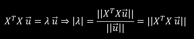
with the second line being a result of the fact that u is assumed unitary. It is therefore obvious that, in order to gauge how the value of λ varies, we must examine the 2-norm (Euclidean norm) of the vector on the right-hand side of the final equals sign.
Let's try unwrapping the product that makes up this vector:
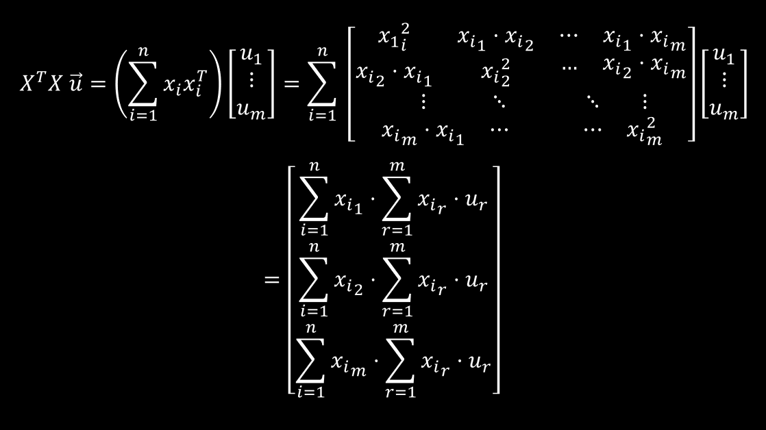
Now, let’s focus on the first element of this vector. If we unwrap it we obtain:

The light blue factors really let us know what’s going on here, since the summations in the parenthesis involve the “filling up” of values in the covariance matrix that lie beyond the main diagonal. For fully correlated data, those values are all zero. On the other extreme, they are all non-zero. It is natural to assume that, as more data arrives, all those values tend to deviate from zero, since some inter-dimensional uncorrelation is, stochastically, bound to occur. On the other hand, if new data is such that it causes an increased inter-dimensional correlation, then the sum will tend towards zero, and the covariance matrix’s spectral norm will actually decrease!
The second vector element deals with the correlation between the second dimension and the rest, and so on and so forth. Therefore, the larger the values of these elements, the larger the value of the 2-norm || X’ X u || is going to be and vice versa.
Some Code
We can demonstrate all this in practice with some MATLAB code. The following function will generate some random data for us:
function X = gen_data(N, s)
%GEN_DATA Generate random two-dimensional data.
% N: Number of samples to generate.
% s: Standard deviation of Gaussian noise to add to the y dimension.
x = rand(N, 1);
y = 2 * x + s.* randn(N, 1); % Adding Gaussian noise
X = [x,y];
end
This function will generate the covariance matrix of the input data and return its spectral norm:
function norm = cov_spec_norm(X)
% COV_SPEC_NORM: Estimate the spectral norm of the covariance matrix of the
% data matrix given.
%   X: An N x 2 matrix of N 2-dimensional points.

COV = cov(X);
[~, S, ~] = svd(COV);
norm = S(1,1).^2;
end
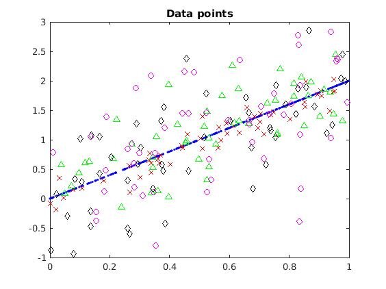
Then we can use the following top-level script to create some initial, perfectly correlated data, plot it, estimate the covariance matrix’s spectral norm, and then examine what happens as we add chunks of data, with increasing amounts of Gaussian noise:
% A vector of line specifications useful for plotting stuff later
% in the script.
linespecs = cell(4, 1);
linespecs{1} = 'rx';linespecs{2} = 'g^';
linespecs{3} = 'kd'; linespecs{4} = 'mo';

% Begin with a sample of 300 points perfectly
% lined up...
X = gen_data(300, 0);
figure;
plot(X(:, 1), X(:, 2), 'b.');  title('Data points'); hold on;
norm = cov_spec_norm(X);
fprintf('Spectral norm of covariance = %.3f.\n', norm)

% And now start adding 50s of noisy points.
for i =1:4
    Y = gen_data(50, i / 5); % Adding Gaussian noise
    plot(Y(:,1), Y(:, 2), linespecs{i}); hold on;
    norm = cov_spec_norm([X;Y]);
    fprintf('Spectral norm of covariance = %.3f.\n', norm);
    X = [X;Y]; % To maintain current data matrix
end
hold off;
(Note that in the script above, every new batch of data gets an inreased amount of noise, as can be seen in the call to gen_data().)
One output of this script is:
>> plot_norms
Spectral norm of covariance = 0.191.
Spectral norm of covariance = 0.200.
Spectral norm of covariance = 0.200.
Spectral norm of covariance = 0.220.
Spectral norm of covariance = 0.275.

Interestingly, in this example, the spectral norm did not change after incorporation of the second noisy data. Can it ever be the case that we can have a decrease of the spectral norm? Of course! We already said that the light blue summations above, corresponding to summations over cells of the covariance matrix beyond the first diagonal, can fall closer to zero after we incorporate new data whose dimensions are more correlated with the existing data’s. Therefore, in the following run, the incorporation of the first noisy set actually increased the amount of inter-dimensional correlation, leading to a smaller amount of covariance (informally speaking).
>> plot_norms
Spectral norm of covariance = 0.177.
Spectral norm of covariance = 0.174.
Spectral norm of covariance = 0.179.
Spectral norm of covariance = 0.220.
Spectral norm of covariance = 0.248.
Discussion
The intuition is clear: as new data arrives in a node, observing the fluctuation of the spectral norm of its covariance matrix can tell us some things about how “noisy” our data is, where “noisiness” in this context is defined as “covariance”. I guess the question to be made here is what to expect of one’s data. If we run a sensor long enough without throwing away archival data vectors, it’s unclear whether we can expect the spectral norm to continuously increase (at least not by a significant margin). We should expect a sort of “saturation” of the spectral norm around a limiting value. This can be empirically shown by a modification of our top-level script, which runs for 50 iterations (instead of 4) but generates batches of data with standard Gaussian noise, i.e the noise does not increase with every new batch:
% Begin with a sample of 300 points perfectly
% lined up...
X = gen_data(300, 0);
norm = cov_spec_norm(X);
fprintf('Spectral norm of covariance = %.3f.\n', norm)

% And now start adding 50s of noisy points.
for i =1:50
    Y = gen_data(50, 1); % Adding Gaussian noise
    norm = cov_spec_norm([X;Y]);
    fprintf('Spectral norm of covariance = %.3f.\n', norm);
    X = [X;Y]; % To maintain current data matrix
end
Notice how the call to gen_data() now adds normal Gaussian noise by keeping the standard deviation static to 1. One output of this script is the following:
>> toTheLimit
Spectral norm of covariance = 0.203.
Spectral norm of covariance = 0.341.
Spectral norm of covariance = 0.388.
Spectral norm of covariance = 0.439.
Spectral norm of covariance = 0.535.
Spectral norm of covariance = 0.635.
Spectral norm of covariance = 0.677.
Spectral norm of covariance = 0.744.
Spectral norm of covariance = 0.818.
Spectral norm of covariance = 0.842.
Spectral norm of covariance = 0.881.
Spectral norm of covariance = 0.913.
Spectral norm of covariance = 0.985.
Spectral norm of covariance = 1.030.
Spectral norm of covariance = 1.031.
Spectral norm of covariance = 1.050.
Spectral norm of covariance = 1.097.
Spectral norm of covariance = 1.148.
Spectral norm of covariance = 1.154.
Spectral norm of covariance = 1.186.
Spectral norm of covariance = 1.199.
Spectral norm of covariance = 1.280.
Spectral norm of covariance = 1.318.
Spectral norm of covariance = 1.323.
Spectral norm of covariance = 1.325.
Spectral norm of covariance = 1.344.
Spectral norm of covariance = 1.346.
Spectral norm of covariance = 1.373.
Spectral norm of covariance = 1.397.
Spectral norm of covariance = 1.447.
Spectral norm of covariance = 1.436.
Spectral norm of covariance = 1.466.
Spectral norm of covariance = 1.466.
Spectral norm of covariance = 1.482.
Spectral norm of covariance = 1.500.
Spectral norm of covariance = 1.498.
Spectral norm of covariance = 1.513.
Spectral norm of covariance = 1.518.
Spectral norm of covariance = 1.518.
Spectral norm of covariance = 1.499.
Spectral norm of covariance = 1.492.
It’s not hard to see that after a while the value of the spectral norm tends to fluctuate around 1.5. Under the given noise model (Gaussian noise with standard deviation = 1), we cannot expect any major surprises. Therefore, if we were to keep a sliding window over our incoming data chunks, and (perhaps asynchronously!) estimate the standard deviation of the spectral norm’s values, we could maybe estimate time intervals during which we received a lot of noisy data, and act accordingly, based on our system specifications.